# Statistical Distributions
This page contains a list of common probability distributions that you may want to use to disperse your inputs in a Monte Carlo analysis. For an overview of common distributions and how they are related, start with this excellent blog post: *[Common Probability Distributions: The Data Scientist’s Crib Sheet](https://medium.com/@srowen/common-probability-distributions-347e6b945ce4)*.
## Usage
# After having initialized your Sim object as 'sim',
# create a continuous uniform random variable between 1 and 5
from scipy.stats import uniform
sim.addInVar(name='var1', dist=uniform, distkwargs={'loc':1, 'scale':4})
## Continuous Distributions
**Uniform Distribution** [[SciPy Ref](https://docs.scipy.org/doc/scipy/reference/generated/scipy.stats.uniform.html), [Wikipedia](https://en.wikipedia.org/wiki/Continuous_uniform_distribution)]:
```uniform(loc, scale)```, where ```loc``` is the lower bound and ```scale``` is size of the range, such that the distribution returns ```x``` from the inclusive range ```[loc, loc + scale]```.
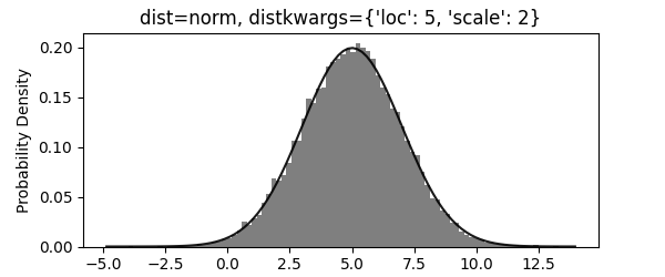
 **Normal Distribution** [[SciPy Ref](https://docs.scipy.org/doc/scipy/reference/generated/scipy.stats.norm.html), [Wikipedia](https://en.wikipedia.org/wiki/Normal_distribution)]:
```norm(loc, scale)```, where ```loc``` is the mean and ```scale``` is the standard deviation. Also known as a Gaussian distribution. The returned range of ```x``` is unbounded. The normal distribution pops up often thanks to the [central limit theorem](https://en.wikipedia.org/wiki/Central_limit_theorem), which states that any distributions when *added* together will tend towards a normal distribution.
**Normal Distribution** [[SciPy Ref](https://docs.scipy.org/doc/scipy/reference/generated/scipy.stats.norm.html), [Wikipedia](https://en.wikipedia.org/wiki/Normal_distribution)]:
```norm(loc, scale)```, where ```loc``` is the mean and ```scale``` is the standard deviation. Also known as a Gaussian distribution. The returned range of ```x``` is unbounded. The normal distribution pops up often thanks to the [central limit theorem](https://en.wikipedia.org/wiki/Central_limit_theorem), which states that any distributions when *added* together will tend towards a normal distribution.
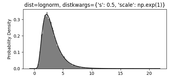
 **Log-Normal Distribution** [[SciPy Ref](https://docs.scipy.org/doc/scipy/reference/generated/scipy.stats.lognorm.html), [Wikipedia](https://en.wikipedia.org/wiki/Log-normal_distribution)]:
```lognorm(s = sigma, scale = numpy.exp(mu))```, where ```mu``` is the mean and ```sigma``` is the standard deviation of the underlying normal distribution. Also known as a Gaussian distribution. Retuns ```x ≥ 0```. Similarly to a normal distribution, this pops up due to the central limit theorem in the log domain, stating that any distributions when *multiplied* together will tend towards a log-normal distribution. Think of stock prices being log-normally distributed when their rate of return is normally distributed.
**Log-Normal Distribution** [[SciPy Ref](https://docs.scipy.org/doc/scipy/reference/generated/scipy.stats.lognorm.html), [Wikipedia](https://en.wikipedia.org/wiki/Log-normal_distribution)]:
```lognorm(s = sigma, scale = numpy.exp(mu))```, where ```mu``` is the mean and ```sigma``` is the standard deviation of the underlying normal distribution. Also known as a Gaussian distribution. Retuns ```x ≥ 0```. Similarly to a normal distribution, this pops up due to the central limit theorem in the log domain, stating that any distributions when *multiplied* together will tend towards a log-normal distribution. Think of stock prices being log-normally distributed when their rate of return is normally distributed.
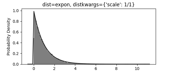
 **Exponential Distribution** [[SciPy Ref](https://docs.scipy.org/doc/scipy/reference/generated/scipy.stats.expon.html), [Wikipedia](https://en.wikipedia.org/wiki/Exponential_distribution)]:
```expon(scale = 1/lambda)```, where ```lambda``` is the expected rate parameter for the associated poisson process. The returned range of ```x``` is unbounded. Think of a call center which receives an average of ```lambda``` calls per minute, and this is the odds of ```x``` minutes passing between subsequent calls.
**Exponential Distribution** [[SciPy Ref](https://docs.scipy.org/doc/scipy/reference/generated/scipy.stats.expon.html), [Wikipedia](https://en.wikipedia.org/wiki/Exponential_distribution)]:
```expon(scale = 1/lambda)```, where ```lambda``` is the expected rate parameter for the associated poisson process. The returned range of ```x``` is unbounded. Think of a call center which receives an average of ```lambda``` calls per minute, and this is the odds of ```x``` minutes passing between subsequent calls.
 ## Discrete Distributions
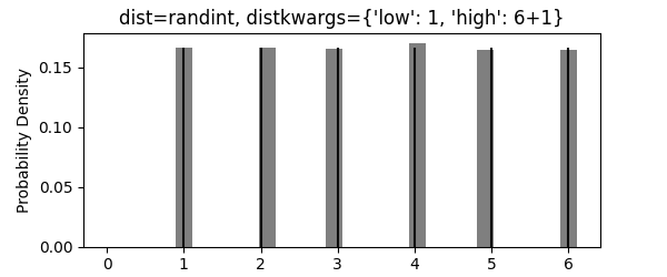
**Random Integers in Range** [[SciPy Ref](https://docs.scipy.org/doc/scipy/reference/generated/scipy.stats.randint.html), [Wikipedia](https://en.wikipedia.org/wiki/Discrete_uniform_distribution)]:
```randint(low, high)```, where ```low``` and ```high``` are the lower and upper bounds of the integer range. Also known as a *discrete* uniform distribution. Returns ```k``` in ```{low, ..., high - 1}```.
## Discrete Distributions
**Random Integers in Range** [[SciPy Ref](https://docs.scipy.org/doc/scipy/reference/generated/scipy.stats.randint.html), [Wikipedia](https://en.wikipedia.org/wiki/Discrete_uniform_distribution)]:
```randint(low, high)```, where ```low``` and ```high``` are the lower and upper bounds of the integer range. Also known as a *discrete* uniform distribution. Returns ```k``` in ```{low, ..., high - 1}```.
 **Random Integers with Custom Weights** [[SciPy Ref](https://docs.scipy.org/doc/scipy/reference/generated/scipy.stats.rv_discrete.html)]:
```rv_discrete(values=(xk, pk))```, where ```xk``` is a list of integers and ```pk``` is a list of the probabilities associated with returning each integer. The sum of ```pk``` must equal 1, and each probability in it must be ```0 < p < 1```. Returns ```x``` in ```xk```.
**Random Integers with Custom Weights** [[SciPy Ref](https://docs.scipy.org/doc/scipy/reference/generated/scipy.stats.rv_discrete.html)]:
```rv_discrete(values=(xk, pk))```, where ```xk``` is a list of integers and ```pk``` is a list of the probabilities associated with returning each integer. The sum of ```pk``` must equal 1, and each probability in it must be ```0 < p < 1```. Returns ```x``` in ```xk```.
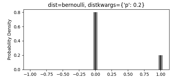
 **Bernoulli Distribution** [[SciPy Ref](https://docs.scipy.org/doc/scipy/reference/generated/scipy.stats.bernoulli.html), [Wikipedia](https://en.wikipedia.org/wiki/Bernoulli_distribution)]:
```bernoulli(p)```, where ```p``` is the probability of success. Equivalent to a "weighted coin flip". Returns ```k``` in ```{0, 1}```.
**Bernoulli Distribution** [[SciPy Ref](https://docs.scipy.org/doc/scipy/reference/generated/scipy.stats.bernoulli.html), [Wikipedia](https://en.wikipedia.org/wiki/Bernoulli_distribution)]:
```bernoulli(p)```, where ```p``` is the probability of success. Equivalent to a "weighted coin flip". Returns ```k``` in ```{0, 1}```.
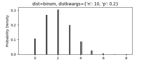
 **Binomial Distribution** [[SciPy Ref](https://docs.scipy.org/doc/scipy/reference/generated/scipy.stats.binom.html), [Wikipedia](https://en.wikipedia.org/wiki/Binomial_distribution)]:
```binom(n, p)```, where ```p``` is the probability of success for a single bernoulli trial, and ```n``` is the number of trials to conduct. Returns ```k``` in ```{0, 1, ..., n}```. Think of the odds of ```k``` heads in ```n``` weighted coin flips.
**Binomial Distribution** [[SciPy Ref](https://docs.scipy.org/doc/scipy/reference/generated/scipy.stats.binom.html), [Wikipedia](https://en.wikipedia.org/wiki/Binomial_distribution)]:
```binom(n, p)```, where ```p``` is the probability of success for a single bernoulli trial, and ```n``` is the number of trials to conduct. Returns ```k``` in ```{0, 1, ..., n}```. Think of the odds of ```k``` heads in ```n``` weighted coin flips.
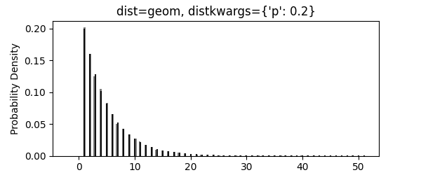
 **Geometric Distribution** [[SciPy Ref](https://docs.scipy.org/doc/scipy/reference/generated/scipy.stats.geom.html), [Wikipedia](https://en.wikipedia.org/wiki/Geometric_distribution)]:
```geom(p)```, where ```p``` is the probability of success for a single bernoulli trial. Returns ```k ≥ 1```. Think of the odds of the number ```k``` of weighted coins you need to flip before you hit heads.
**Geometric Distribution** [[SciPy Ref](https://docs.scipy.org/doc/scipy/reference/generated/scipy.stats.geom.html), [Wikipedia](https://en.wikipedia.org/wiki/Geometric_distribution)]:
```geom(p)```, where ```p``` is the probability of success for a single bernoulli trial. Returns ```k ≥ 1```. Think of the odds of the number ```k``` of weighted coins you need to flip before you hit heads.
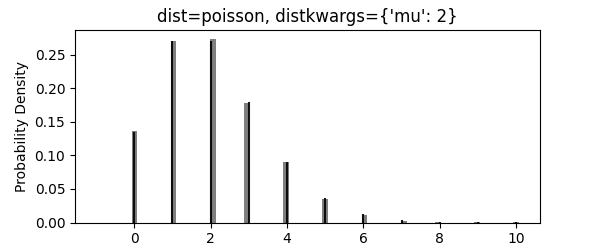
 **Poisson Distribution** [[SciPy Ref](https://docs.scipy.org/doc/scipy/reference/generated/scipy.stats.poisson.html), [Wikipedia](https://en.wikipedia.org/wiki/Poisson_distribution)]:
```poisson(mu)```, where ```mu``` is the expected rate of occurances (notated as lambda on wikipedia). Returns ```k ≥ 0```. Think of a call center that receives an average of lambda calls per minute, and this gives the odds of receiving ```k``` calls in any given minute.
**Poisson Distribution** [[SciPy Ref](https://docs.scipy.org/doc/scipy/reference/generated/scipy.stats.poisson.html), [Wikipedia](https://en.wikipedia.org/wiki/Poisson_distribution)]:
```poisson(mu)```, where ```mu``` is the expected rate of occurances (notated as lambda on wikipedia). Returns ```k ≥ 0```. Think of a call center that receives an average of lambda calls per minute, and this gives the odds of receiving ```k``` calls in any given minute.